OTA 2018 Debrief: Cornering Compliances and Transients
2019/08/22 update: this article is part of a series on on-centre vehicle handling using linear system analysis. For further reading, please feel free to check out my other posts:
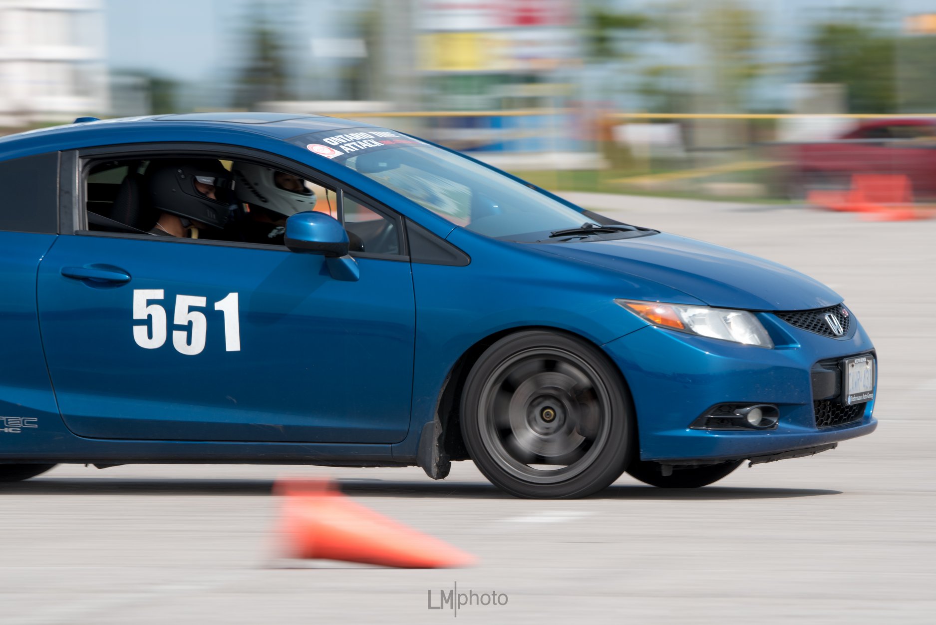
Photo Credit: Michael Lim
Welcome to the Ontario Time Attack debrief files, a series of articles where we answer vehicle dynamics questions we always wanted to ask, but could not tackle during the racing season. In this instalment, we perform a pulse steer test to identify vehicle handling properties.
Transient Handling
The understeer gradient is a measure of steady-state vehicle handling. However, in order to wholistically evaluate handling performance, it is necessary to analyze both steady-state and transient vehicle responses.
The linear single-track vehicle provides a foundational model to study on-centre vehicle handling. System identification allows analytical examination of handling properties in both steady-state and transient maneuvers.
Understeer, Defined
In our last article, we defined understeer as the tendency for a vehicle to require more (or less) steering input relative to the Ackermann steer angle. The gain due to lateral acceleration is the understeer gradient.
\[\delta = \frac{L}{R} + K a_y\]Where:
- \(\delta\) is the steering angle [\(rad\)]
- \(L\) is the wheelbase of the car [\(m\)]
- \(R\) is the radius of the turn [\(m\)]
- \(a_y\) is the lateral acceleration [\(m/s^2\)]
- \(K\) is the understeer gradient [\(\frac{rad}{m/s^2}\)]
Equivalently, the understeering tendency can be described as the difference in the front and rear slip angles.
\[\delta = \frac{L}{R} + (\alpha_f - \alpha_r)\]Where:
- \(\alpha_f\) represents the front axle effective slip angle [\(rad\)]
- \(\alpha_r\) represents the rear axle effective slip angle [\(rad\)]
Combining both definitions of understeer yields the following relationship:
\[K = \frac{1}{a_y} (\alpha_f - \alpha_r)\]We assume that the front and rear axles experience the same lateral acceleration, \(a_y\). Equating the tire force to lateral acceleration experienced by each axle yields the following relationship:
\[m_f a_y = \alpha_f C_f\] \[m_r a_y = \alpha_r C_r\]Where:
- \(m_f\) represents the equivalent mass of the front axle [\(kg\)]
- \(m_r\) represents the equivalent mass of the rear axle [\(kg\)]
- \(C_f\) represents the front axle effective cornering stiffness [\(N/rad\)]
- \(C_r\) represents the axle axle effective cornering stiffness [\(N/rad\)]
Rearranging and solving for the front and rear slip angles:
\[\alpha_f = \frac{m_f a_y}{C_f}\] \[\alpha_r = \frac{m_r a_y}{C_r}\]Substituting the front and rear slip angles yields the following definition of the understeer gradient.
\[K = \frac{m_f}{C_f} - \frac{m_r}{C_r} = D_f - D_r\]Where:
- \(D_f\) represents the front axle cornering compliance [\(\frac{rad}{m/s^2}\)]
- \(D_r\) represents the rear axle cornering compliance [\(\frac{rad}{m/s^2}\)]
The understeer gradient can therefore be understood as the difference between the front and rear cornering compliances. This definition is mathematically consistent with the earlier definition of the understeer gradient. Noteworthy of mention is the exclusion of the steer angle term in the cornering compliance definition of the understeer gradient.
Experimental Setup
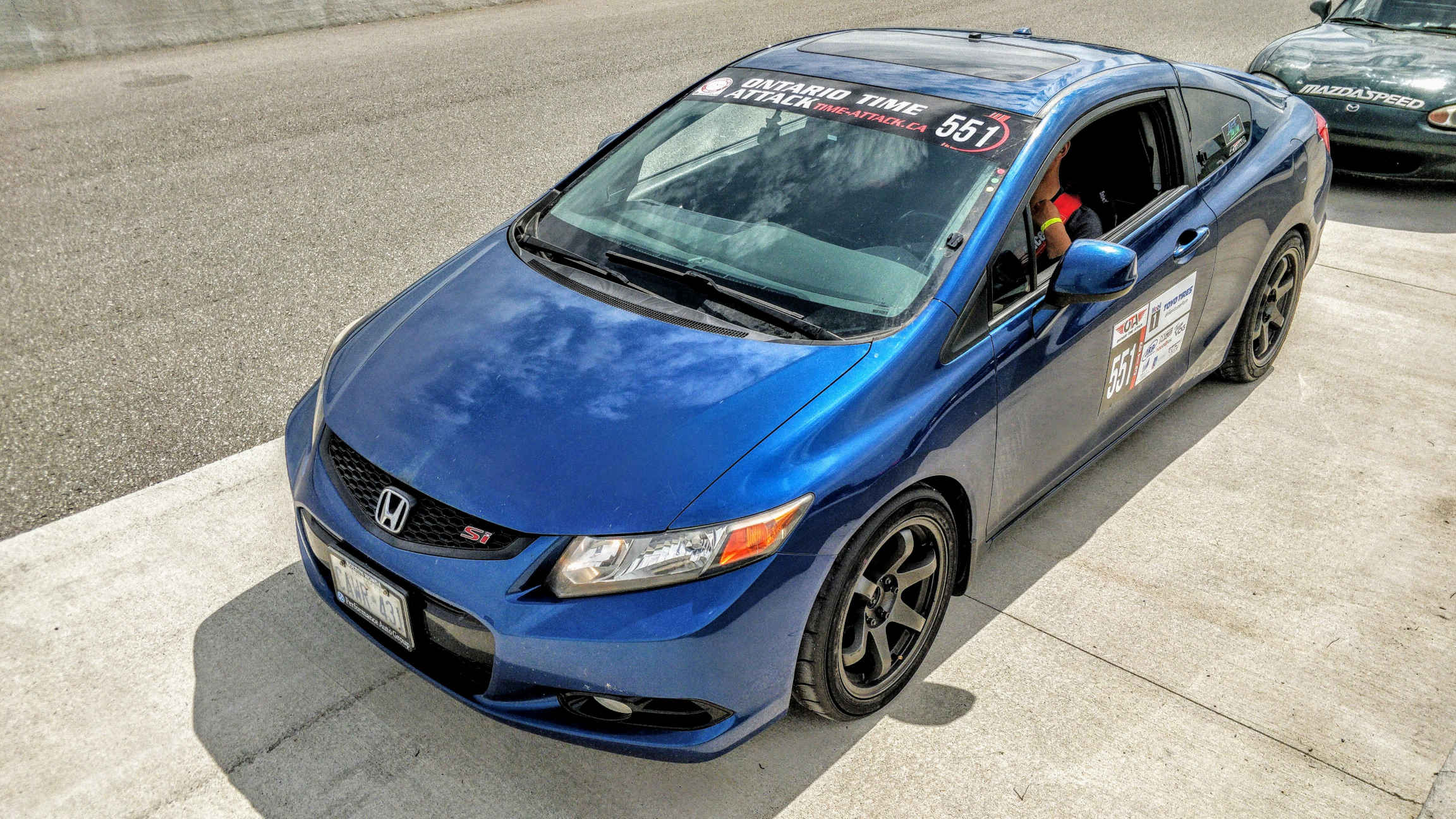
The target vehicle is a 2012 Honda Civic Si Coupe equipped with adjustable coilovers, staggered wheel sizing, bucket racing seat and roll bar. All data is collected with an Autosport Labs RaceCapture/Pro Mk2 data acquisition system. The data acquisition system is connected to the vehicle via the diagnostics port.
The pulse steer test consists of driving straight ahead at constant speed, ‘pulsing’ the steering wheel by rapidly steering to a non-zero steer angle and returning the steering to centre.
The pulse steer test is performed on a flat testing area of a race track. This test is performed off the active track and in a designated testing area.
A test speed of 30 km/h is chosen for safety purposes. The duration of a pulse steer test is very short; a single test is less than 2 seconds in duration.
The test is performed immediately after leaving the active track such that the tire temperatures and tire pressures are similar to those seen in racing conditions.
Safety is of utmost concern. At no time did the vehicle operate outside the scope of driver control, and at no time did the driver operate the vehicle in an unsafe manner. Do not perform this test in an uncontrolled area.
Vehicle Parameters
The following vehicle parameters are assumed for the vehicle-under-test:
| Symbol | Value | Unit | Description |
|---|---|---|---|
| \(a\) | 0.996 | m | Distance from CG to front axle |
| \(b\) | 1.624 | m | Distance from CG to rear axle |
| \(m\) | 1450 | kg | Vehicle mass |
| \(I\) | 2345 | kg m2 | Vehicle yaw inertia |
| \(K\) | 5.5 | deg/g | Understeer gradient (as measured) |
Results
The system identification yields the following cornering compliances:
- \(D_f = 9.6\) [deg/g]
- \(D_r = 4.1\) [deg/g]
The difference between the front and rear cornering compliances yields the understeer gradient:
\[K = D_f - D_r = 5.5\ [deg/g]\]The following graph shows the simulated response plotted against the experimental data acquired from in-vehicle testing.
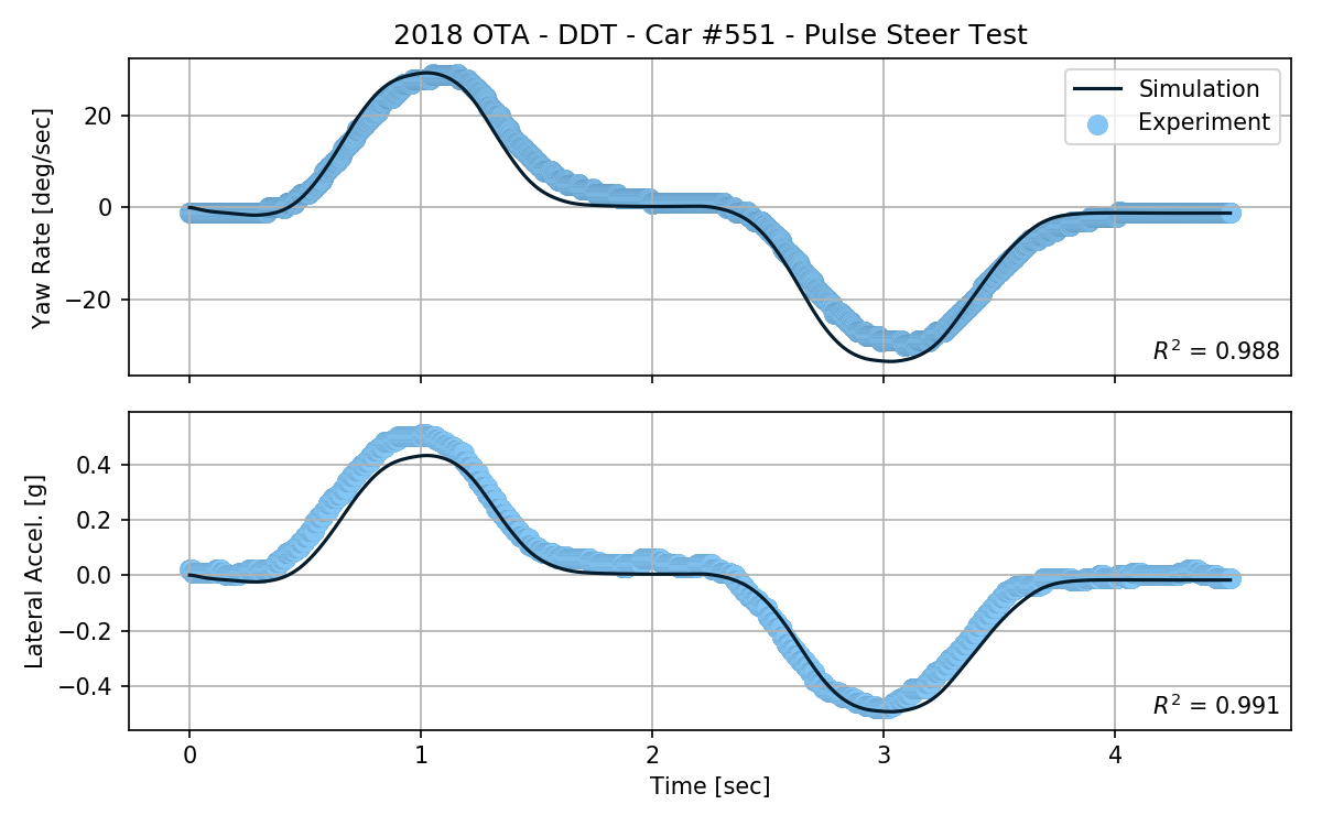
The simulation over-predicts the yaw acceleration of the vehicle in comparison to the experimental data. However, the model matches the peak yaw rate of the experimental data quite well. Peak lateral acceleration is under-predicted in the positive case, but correlates well in the negative case.
To validate the model, on-track data from another session is compared against the simulation. The chosen validation dataset is of a warmup lap at Toronto Motorsports Park, turns 7 & 8. The vehicle speed is near constant at approximately 80 km/h.
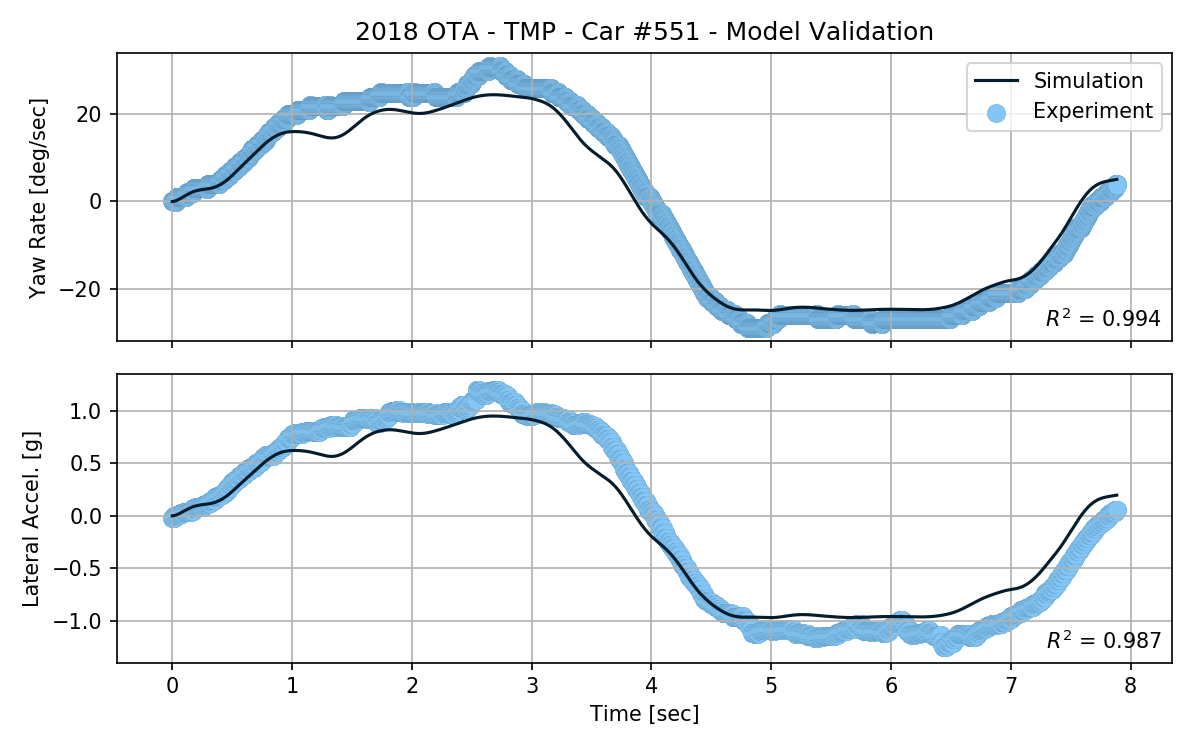
The simulation under-predicts the peak lateral acceleration by approximately 20% in both directions. Yaw rate is well predicted in the negative case, but is under-predicted in the positive case.
Summary
The purpose of performing the pulse steer test is to identify the front and rear cornering compliances of the vehicle. Combined with the understeer gradient test, a simple transient vehicle model is developed.
Simulation and modelling enables analytical insight into vehicle handling. The simulation is not without caveats; the simulation does not perfectly capture the transient response of the vehicle observed the experimental data. Despite these pitfalls in the accuracy of the simulation, the model has enough fidelity to provide useful information about the vehicle. The ability to generalize the vehicle response in a simulation is still an extremely powerful tool in analyzing and assessing handling performance.
A big thank you to OTA competitor Joseph Yang in the #551 2012 Honda Civic Si for performing the pulse steer test and for providing the data used the analysis. This article would not be possible without the support of Joseph Yang and his sponsors.
References
- Milliken, William F., and Douglas L. Milliken. Race car vehicle dynamics. Vol. 400. Warrendale: Society of Automotive Engineers, 1995.
- Dixon, John. Tires, suspension and handling. SAE, 1996.
- Bundorf, R. Thomas, and Ronald L. Leffert. The cornering compliance concept for description of vehicle directional control properties. No. 760713. SAE Technical Paper, 1976.
- Testing, Testing 1,2 …” FSAE.com, 2015, www.fsae.com/forums/showthread.php?12204-Testing-Testing-1-2-…